Authors: Natalie Pearson
It is a truth universally acknowledged that a person in possession of a quantum computer must be in want of a use for it. When to use quantum computing and what to use it for are icebreaking conversation topics, certain to add some spice to an otherwise flavourless dinner party. There are many considerations to be taken into account, starting with identifying an interesting and useful problem.
We know that there are some problems which very quickly become intractable for classical computers and where quantum computers already outperform them, however, it remains a lively debate as to whether these instances constitute a “practical quantum advantage”. In this series of blog posts we addressed the question of when to use a quantum computer at all (still a very debated topic). Usually instances where quantum computers can outperform classical computers involve operating the quantum computer in analog mode and using it to simulate another quantum system. There are two modes or paradigms of quantum computing: digital and analog, each with its own benefits and drawbacks, and where a single underlying hardware can often be operated in either mode, as at Pasqal.
The Quantum Mountaineer’s Dilemma: Which Route to the Summit?
The analog mode of quantum computers leverages the natural evolution of the quantum system to implement algorithms, which typically requires little overhead in terms of compilation. The major drawbacks are that this significantly limits the scope of problems that can be solved (essentially only problems that can be mapped onto the specific hardware in analog mode) and, without access to error correction schemes, the errors in the system accumulate, so that it becomes harder and harder to obtain accurate results as the scale of the problem increases. The digital mode of quantum computers relies on algorithms being described by discrete gate operations which are precalibrated on the hardware. These have the benefit of universality (meaning they can be used to implement any algorithm) and the possibility to make use of the many error correction schemes so that they can avoid the problem of errors accumulating. This comes at the cost of a large overhead, both in terms of number of qubits required, total runtime, and complexity of the algorithm.

Imagine that, an intrepid quantum mountaineer has secured a quantum device and identified a particular challenge of interest. She is now presented with another choice on her quest; which path to take. Ideally she would have access to the knowledge of which path requires less resources and will enable her to most quickly and with success reach the summit (and solve the problem).
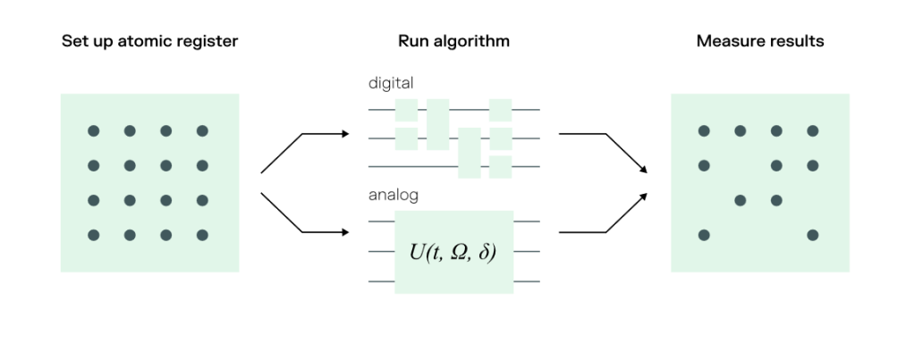
In order to compare the two modes, to facilitate this decision, we choose the example of a problem with an algorithm known to be performant on our neutral atom quantum hardware in analog mode, and explore how performant running it in digital mode would be. To skip straight to the punchline, the information that would have helped our quantum mountaineer is shown below. For a certain choice of mountain (algorithm) the intrepid mountaineer (QPU user) can determine which route (mode) to use. This will depend on the date of their adventure (which version of Pasqal’s QPU they have access to) and the equipment available to them (how many logical gates are available in digital mode).

Using the method described below we can determine the number of logical gates and qubits needed to compete with different analog implementations on the Pasqal roadmap at the chosen algorithm. These results, shown above, are based on the physical capabilities of Pasqal’s devices, with sizes ranging from 100 qubits in 2024 to 1000 in 2028. What we can see is that, at this specific task, the analog mode will outperform the digital mode until large numbers of logical gates are able to be performed. These results also emphasise the importance of developing fault tolerant, error corrected digital schemes, as the implementation of these will be necessary in order to go beyond the capabilities of analog and fully realise the potential of quantum computing for a wide range of applications. By providing both modes of quantum computation at Pasqal using the same underlying hardware, we facilitate near term applications, while also building for the future.
For the details of how we did this, and to really make an impression on your fellow dinner guests (good or bad we cannot say), read the next section.
Technical Breakdown: Cartography for the quantum mountaineer
As an algorithm we choose the simulation of quench dynamics. This involves mimicking the behaviour of a quantum system of interest left to evolve out of equilibrium and can tell us about properties of the system, which we might otherwise not have controlled access to. For example, by mimicking how electrons move in a material when it’s heated or disturbed, we can uncover hidden quantum behaviours that are difficult to access through direct measurement. There is precedent for this being one of the most promising avenues for quantum advantage, as it most closely aligns with what analog quantum hardware is good at and is intrinsically hard to simulate classically. In order to quantify how good our neutral atom quantum hardware would be at this task we implement the algorithm perfectly by emulating it without noise to obtain the ideal result and then repeat the implementation using the analog mode of a realistic quantum device (i.e with noise). We choose an observable to measure and compare the value at the end of the simulations to the true value obtained without noise. This enables us to quantify how “well” our realistic device performs. We call the difference between the true value and the value from the realistic analog device the error budget.
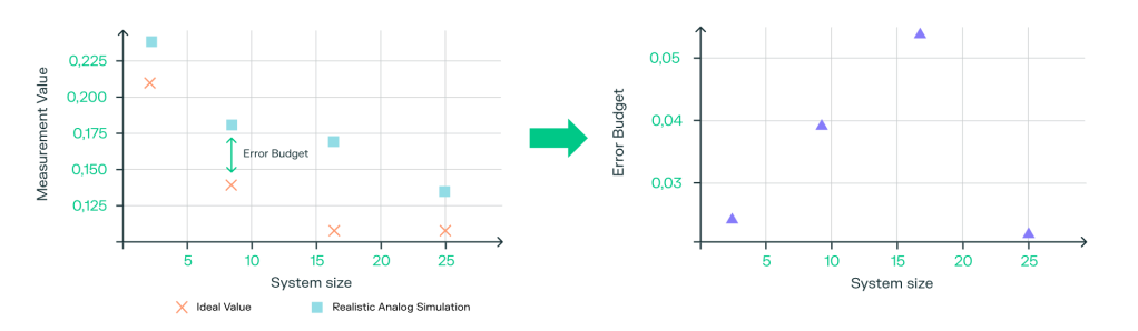
In order to implement the same algorithm using digital mode we first have to ‘digitise’ the algorithm. This is done by a method called the Trotter-Suzuki decomposition, which is a way to break down an evolution into many single and two qubit gates which implement small time slices of the evolution and, when put together, induce the same dynamics in the system as the analog version. It is possible to increase the accuracy of this method by increasing the number of gates used. We choose to assume perfect logical gates with ideal connectivity and only include the error from the digitization process, finding the number of gates needed to achieve the same error budget as our realistic analog device achieves. This tells us that, until we can implement this many gates very well, we are better off using the analog device for this implementation.
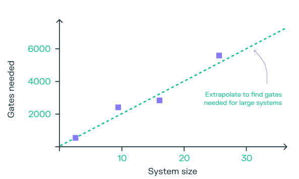
Armed with our algorithm and our three implementations (perfect, realistic-analog and Trotterised-digital) we are ready to go. We find the error budget using the first two implementations and, using our third implementation, the number of gates required to match this. It is only possible to do this using small systems which we are able to simulate classically (exactly because of the fact that we’ve chosen an algorithm that classical computers find hard!). We run simulations for small systems of different sizes, using the corresponding number of qubits for the simulation, to find the number of gates needed for each size. From this we can determine the relation between the system size and the number of gates needed and hence calculate how many gates we would need for larger system sizes, beyond classical simulation capabilities. Systems of this size are already realised at Pasqal, as described in this previous blog post. In the end, if the quantum mountaineer has chosen the mountain corresponding to simulating a quantum quench, then, if she knows how many perfect logical gates she has available to her and the date of the expedition, she can find which path to take by looking at the main figure to find her ‘location on the map’ which tells her which path (mode) to take. It’s very likely to be the analog one!

Expert Corner: Assumptions and Obstacles on the path
In the interest of brevity (and storytelling) we have of course left out some of the details here which in turn will have an impact on the values and reliability of the results. For full transparency we note the main decisions and implications here:
- This result will be different for different problems and different observables, we chose a quantum Ising-like quench as this is the native Hamiltonian of the Rydberg atom system. We chose the measured value to be a two point correlator between the centre and corner atoms, behaviour was similar for other two point correlators
- The results are specific to the assumed error model(s) of the analog system as lower analog errors will decrease the error budget and hence require more digital gates to reach the same budget. We have used the current generation error model and the expected model for our future generations of devices. Improvements in the analog hardware may increase the gate counts required.
- From the perfect (logical) gates figure you’ll see that we have data only for small systems and have used it to make estimates about much larger systems. The feasibility of this extrapolation is likely to be the largest source of uncertainty in our calculations
- We have assumed our digital gates and qubits to be perfect. Realistically this requires logical gates and qubits and use of error correction. In order to obtain estimates for the number of physical qubits and gates needed we would need to make an assumption about which fault tolerant scheme is being used in order to calculate the resulting overhead in physical gate and qubit numbers, which are typically significant. Alternately we could assume no error correction and that these gates are physical but then we would need to include realistic digital gate errors in our simulations which would reduce the accuracy of the digital mode.
- We have assumed full connectivity of the digital implementation. In practice realistic (reduced) connectivity will add further overhead in gate counts.
- We have not worked hard to optimise the digital circuit (i.e we have built the digital circuit to implement the algorithm in the simplest way (1st order Trotter)), we may be able to reduce the amount of digital resources required if we optimised this further.