
Partial differential equations and finite elements
Differential equations describe the interrelationships between various quantities in a system and their rates of change. These equations are ubiquitous in the physical sciences, engineering and human-made systems. They can be used to describe phenomena ranging from elasticity to aerodynamics, from epidemiology to financial markets. Exact solutions are rare, and solving these equations often involves using numerical techniques consuming enormous computational resources.
The class of finite element methods (FEM) include the most widely used techniques to solve differential equations numerically. The idea behind such methods is to treat space and time as discrete and replace continuous rates of change with stepwise differences. The FEM has become the de-facto approach to deal with complex differential equations in industry and research. Its use is so widespread that it underpins a multi-billion dollar simulation software market with double-digit annual growth. But FEMs suffer from important limitations. Most notably, FEMs are rigid and unable to exploit observational data.
Bringing equations and data together
Generally, engineers and researchers are not solving differential equations for its own sake but to understand real-world phenomena. Whether solving differential equations is the right approach depends on the availability of observational data. If data is scarce, but we understand the underlying dynamics in detail, then solving differential equations using FEM is the natural approach. On the other hand, if we have copious amounts of data but ignore the equations that govern the system, the question is more amenable to machine learning techniques.
In practice, most problems lie somewhere in between: we have some data and a partial understanding of the underlying physics.
We should therefore aim at developing methods suited for this intermediate situation. The problem is that observational data cannot be incorporated into FEM solvers or workflows in a straightforward fashion. This forces us to choose between first principles- and data-driven approaches. But a new approach is emerging. A new paradigm, known as physics-informed machine learning (PIML), aims at integrating data and first principles seamlessly [1]. This new approach could pave the way for new solvers that place equations and data on the same footing.
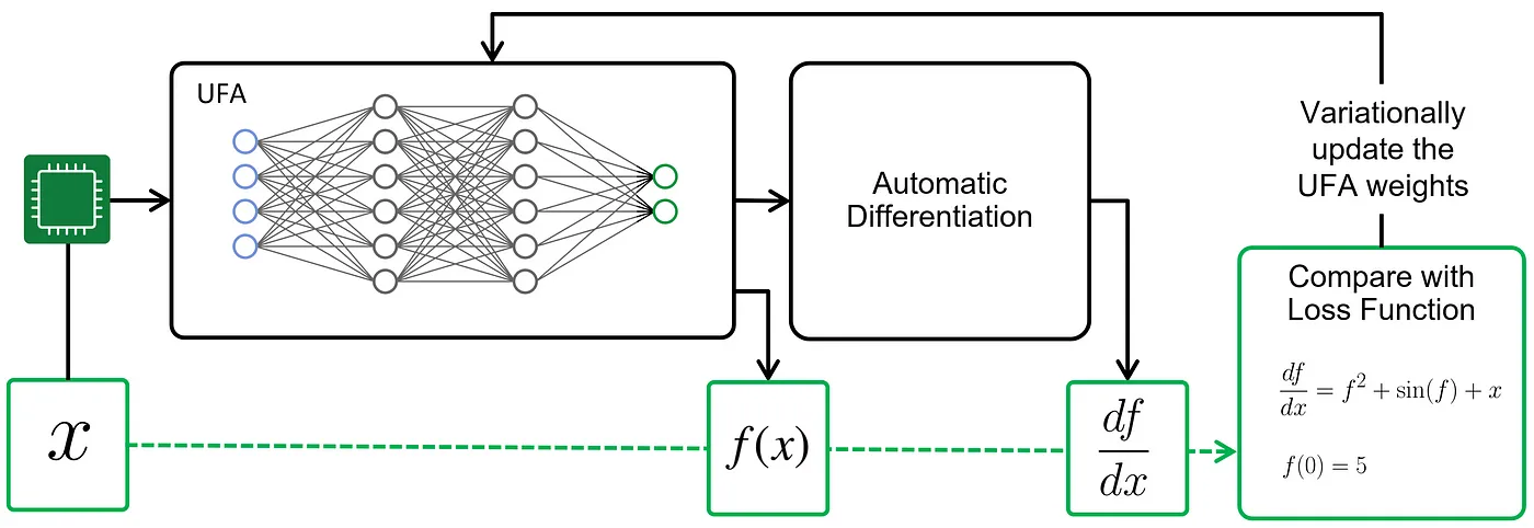
The core idea behind PIML is simple. The core task in machine learning is to train an agent for making accurate predictions. The first step is to introduce a loss function measuring how far off are the agent’s predictions. The learning process consists of gradually adjusting the agent’s parameters to improve its predictions. In standard machine learning, the loss function and training are based on data.
In PIML, the loss function and training also consider the physical laws governing the system: the differential equation itself, and the boundary and initial conditions. PIML loss functions grade an agent’s predictions not only on how close they are to the data but on whether they are consistent with the governing equations (Fig. 1). This opens attractive new strategies where data and dynamics can be used in complementary ways.
Universal function approximators
The main ingredient of any PIML method is a universal function approximator (UFA). This is a parameterized function that can be used to approximate, or ‘fit’, a solution to the differential equation at hand: the speed of a fluid, a temperature distribution, etc. By design, a UFA comes with trainable parameters that are tuned by the training process. A UFA must satisfy two requirements. First, it should have enough ‘expressivity’ or capacity to approximate the solution for a differential equation. Second, we should be able to efficiently calculate the UFA’s rates of change with respect to space and time, and the trainable parameters.
There are many possible choices for the UFA, ranging from polynomials with tunable coefficients to Fourier series. Today, the most popular and well-known UFAs are deep artificial neural networks, whose rates of change are efficiently computed using automatic differentiation.
We are still on the early days, but it is clear that PIML opens several interesting possibilities:
- Multi-physics problems: Given that the UFAs are efficiently differentiable, PIML can easily incorporate multiple differential equations, complex boundary conditions, and interface conditions, making them suitable for a wide variety of multi-physics problems.
- No mesh required: The UFA does not need to be evaluated on a complex mesh such as those used for FEM; instead, a cloud of points extracted randomly from the chosen domain is sufficient and repeated sampling over the optimization procedure effectively mitigates the risk of overfitting.
- Experimental feedback: In contrast to FEM, it is easy to incorporate experimental observations of the physical system under study. These observations are simply treated as known data points and added to the loss function, thereby directly improving the training efficiency.
- Digital twins: Once the UFA is optimized on a particular physical system, the properties of a similar system with different geometrical parameters or boundary conditions can be inferred without the re-execution of the whole simulation. This makes the PIML approach suitable for applications such as product design or digital twins, where a large number of different configurations of the same system must be evaluated very quickly.
In our view, the most attractive feature of PIML-based techniques is their potential to harness the computational advantage given by quantum computers. PASQAL recently demonstrated how PIML techniques can be seamlessly ported to the quantum realm by using a quantum neural network as the UFA. To learn more, have a look at our post on differentiable quantum circuits and their implementation on PASQAL’s neutral atom platform.
Conclusion
Given these benefits, we believe that PIML techniques are poised to become a crucial ingredient in any differential equation solver toolbox. To support this claim, we will regularly publish new posts applying the PIML techniques outlined here in combination with quantum computation on industrially-relevant problems governed by differential equations.
Stay tuned!
[1] M.Raissi, P.Perdikaris, G.E.Karniadakis (2019). Physics-informed neural networks: A deep learning framework for solving forward and inverse problems involving nonlinear partial differential equations. Journal of Computational Physics, Volume 378.
The main contributing authors to this blog are Evan Philip, Mario Dagrada and Vincent Elfving.